Faculty Datasets
Contents
Datasets is Faculty’s environment for storing large files. It is designed to prevent accidental loss or modification of important data. Before proceeding, you may want to skim through the tutorial on Accessing Data.
To access the Datasets environment, click the relevant icon in the tab on the
left-hand side of the workspace. Once inside the Datasets environment, the
buttons on the top-right of the page offer three options, Upload file,
Create folder, and Delete file. It is important to note that other actions,
such as moving files from Datasets to the workspace, can be performed using
the faculty.datasets Python module.
Files uploaded to Datasets in CSV or TSV format are automatically analysed with Lens, Faculty’s data-exploration service. As we will see, reports generated by Lens can be readily accessed from the Datasets page. If, on the other hand, you would like to use this feature as a Python module, find its documentation here.
Lens reports evaluate the quality of datasets, and offer immediate insight through visualisations and tabular summaries.
Moving files to and from datasets
In order to move files from Datasets to the workspace, where you can use files in your programs, we provide a Python and R library that lets you manipulate files on Datasets.
The Python library is called faculty.datasets. To save you some
typing, you can import it as datasets:
import faculty.datasets as datasets
You can then use the commands as follows:
datasets.put('/project/test-file.csv', '/input/test-file.csv')
The various functions for manipulating files are:
|
Copy a file or directory within a project’s datasets. |
|
Get a unique identifier for the current version of a file. |
|
Copy from a project’s datasets to the local filesystem. |
|
List contents of project datasets that match a glob pattern. |
|
List contents of project datasets. |
|
Move a file or directory within a project’s datasets. |
|
Open a file from a project’s datasets for reading. |
|
Copy from the local filesystem to a project’s datasets. |
|
Remove a file or directory from the project directory. |
|
Remove an empty directory from the project datasets. |
To find a full list, take a look at the faculty.datasets page.
The R library is called rfaculty. As always, we load it with the library command:
library(rfaculty)
You can then use the commands as follows:
datasets_put('/project/test-file.csv', '/input/test-file.csv')
The various functions for manipulating files are:
datasets_get(datasets_path, local_path, project_id = NULL)Copy from the Faculty datasets to the local filesystem.
datasets_move(source_path, destination_path, project_id = NULL)Move a file from one location to another on Faculty Datasets.
datasets_delete(path, project_id = NULL)Delete a file from Faculty Datasets.
datasets_list(prefix = “/”, project_id = NULL, show_hidden = FALSE)List files on Faculty datasets.
datasets_copy(source_path, destination_path, project_id = NULL)Copy a file from one location to another on Faculty Datasets.
datasets_etag(path, project_id = NULL)Retrieve the etag for a file on Faculty datasets.
datasets_put(local_path, datasets_path, project_id = NULL)Copy from the local filesystem to Faculty datasets.
Note
Copying and moving large files (> 1 GB) is currently not well supported. Instead of using the cp and mv commands, consider downloading the file first, and re-upload it to a different location within datasets. Then, remove the original file if needed.
Lens reports
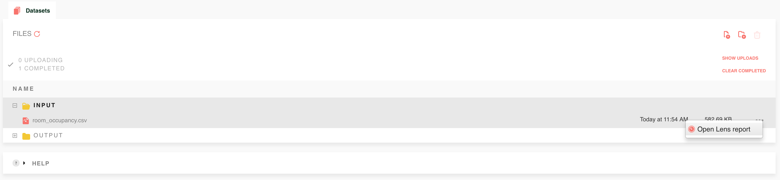
Within the Datasets environment, select the CSV or TSV file you that would
like to explore. The icon  on the right-hand side of the page will direct
you to the Lens report.
on the right-hand side of the page will direct
you to the Lens report.
Interpreting Lens reports
Your Lens report will typically look like this:
Lens reports are organised in three parts, namely Columns, Correlation Matrix and Pairwise Density Plot. Each corresponds to a tab, so that you can navigate through a report as you would in your web browser.
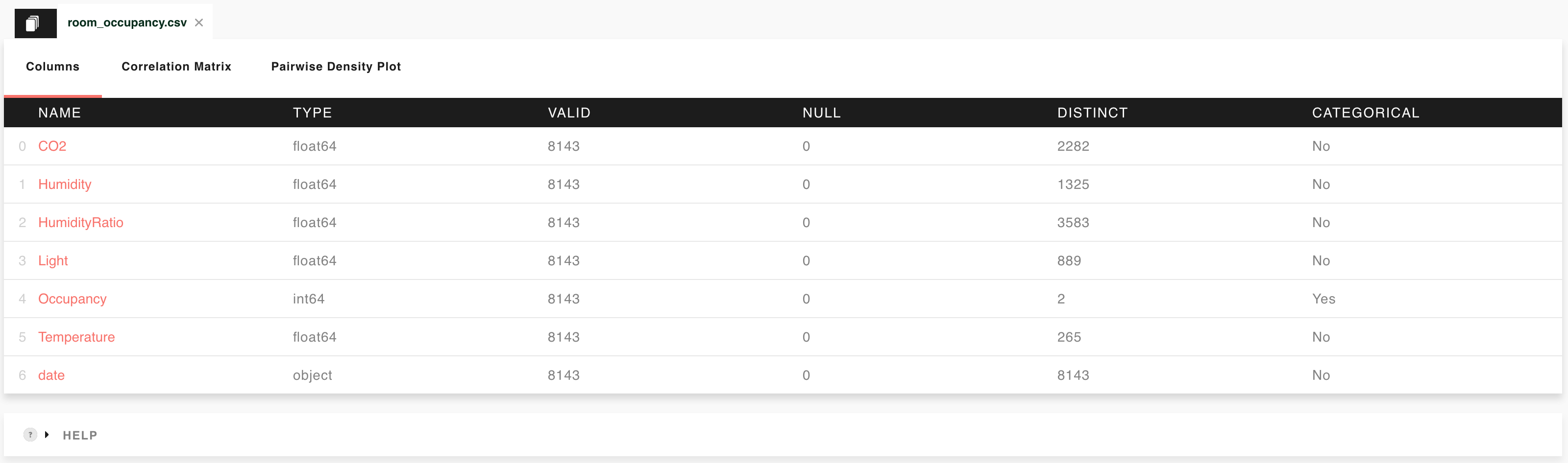
Columns
This is the “landing page” of the report. It lists the quantities (Columns) found in the dataset, alongside their main characteristics,
TYPE: the way the column is encoded. As in the data-analysis tool Pandas, the type can be
int64(integer number),float64(floating point number), orobject(non-numeric).VALID: the number of non-null entries in the column.
NULL: the number of null entries in the column. The sum of VALID and NULL is equal to the size of your dataset.
DISTINCT: the number of distinct entries in the column. In other words, repeated identical values are counted only once.
CATEGORICAL: If
No, the column is numeric (int64orfloat64). Else the column is non-numeric (object).
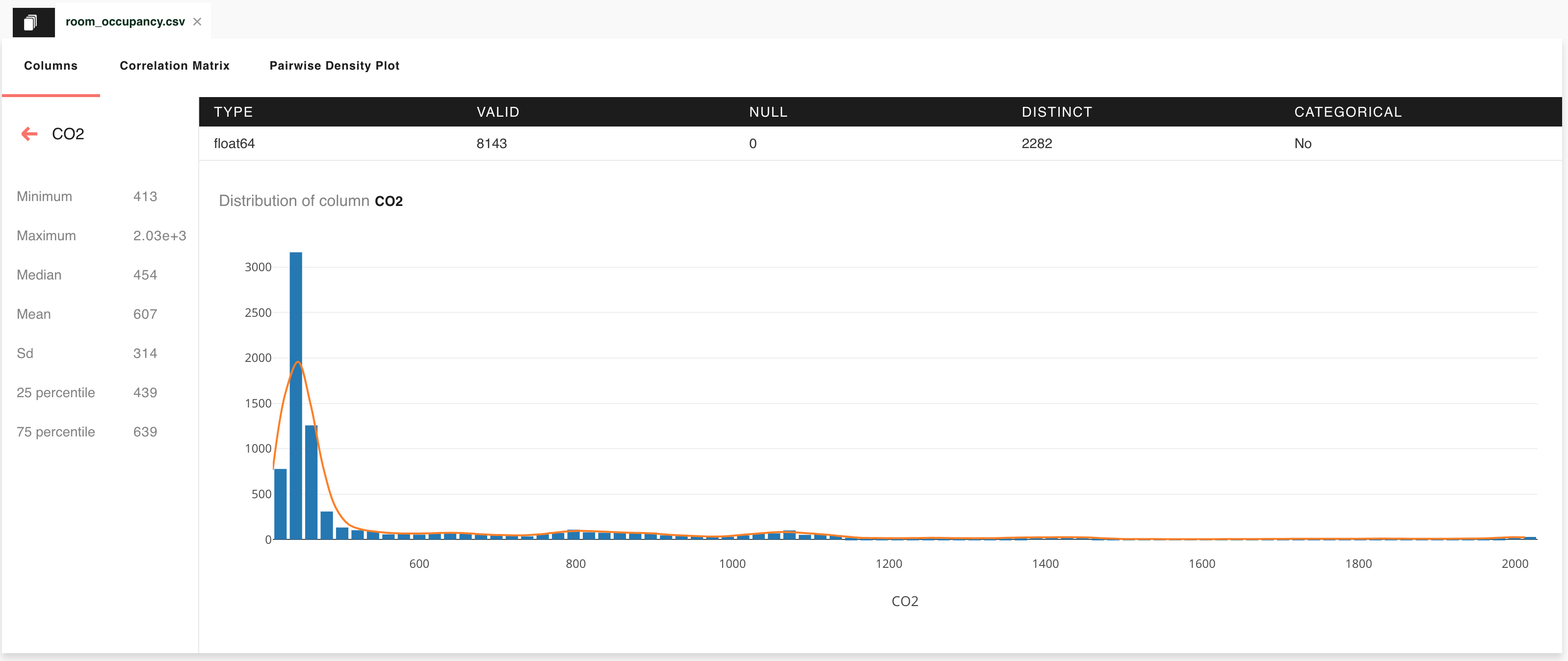
Note
Clicking the name of a numeric quantity will direct you to the corresponding histogram. The plot will also include an estimate of the Probability Density Function (PDF) for the quantity, represented as a solid yellow line. More precisely, Lens calculates the PDF by means of a kernel density estimation (KDE) method.
Correlation matrix
Data scientists are often interested in correlations, as these indicate whether it is possible to make predictions. For example, let us assume the score of pupils in a test is highly correlated with the number of hours they studied. Then, given a pupil who has never taken the test, the number of hours he/she spent studying can be used to predict his/her score.
Lens calculates the correlation coefficient of each quantity in the dataset with all the others, and reports back a correlation matrix that summarises this information. For instance, each diagonal entry of this matrix specifies the correlation coefficient of a quantity with itself, which is equal to 1 by definition.
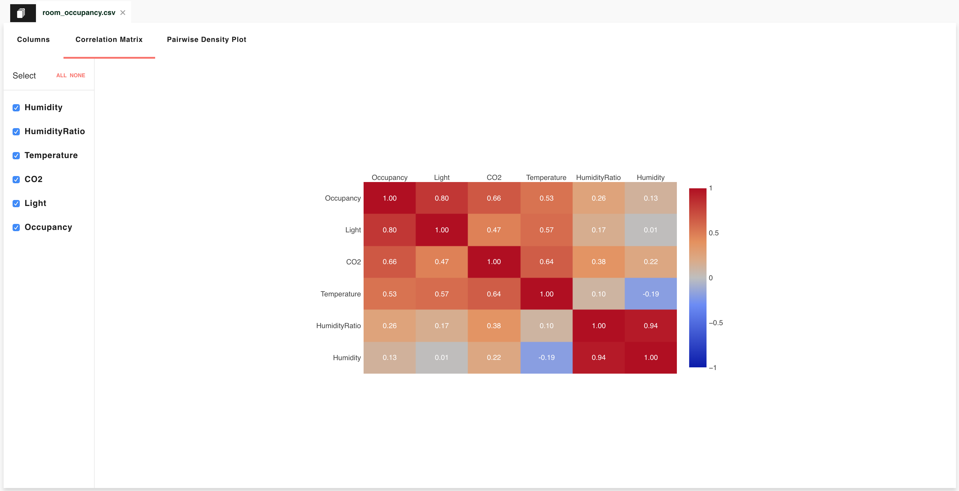
More technically, Lens returns the Spearman rank-order correlation coefficient matrix for your dataset.
Pairwise density plot
To better characterise the correlation between two quantities, it is useful to create a scatter plot. The tab Pairwise Density Plot in your Lens report displays, in a sense, all scatter plots that can be generated by examining the quantities in the dataset pairwise. Whenever a quantity is compared with itself, the scatter plot conveys no information, and thus a histogram is displayed instead.
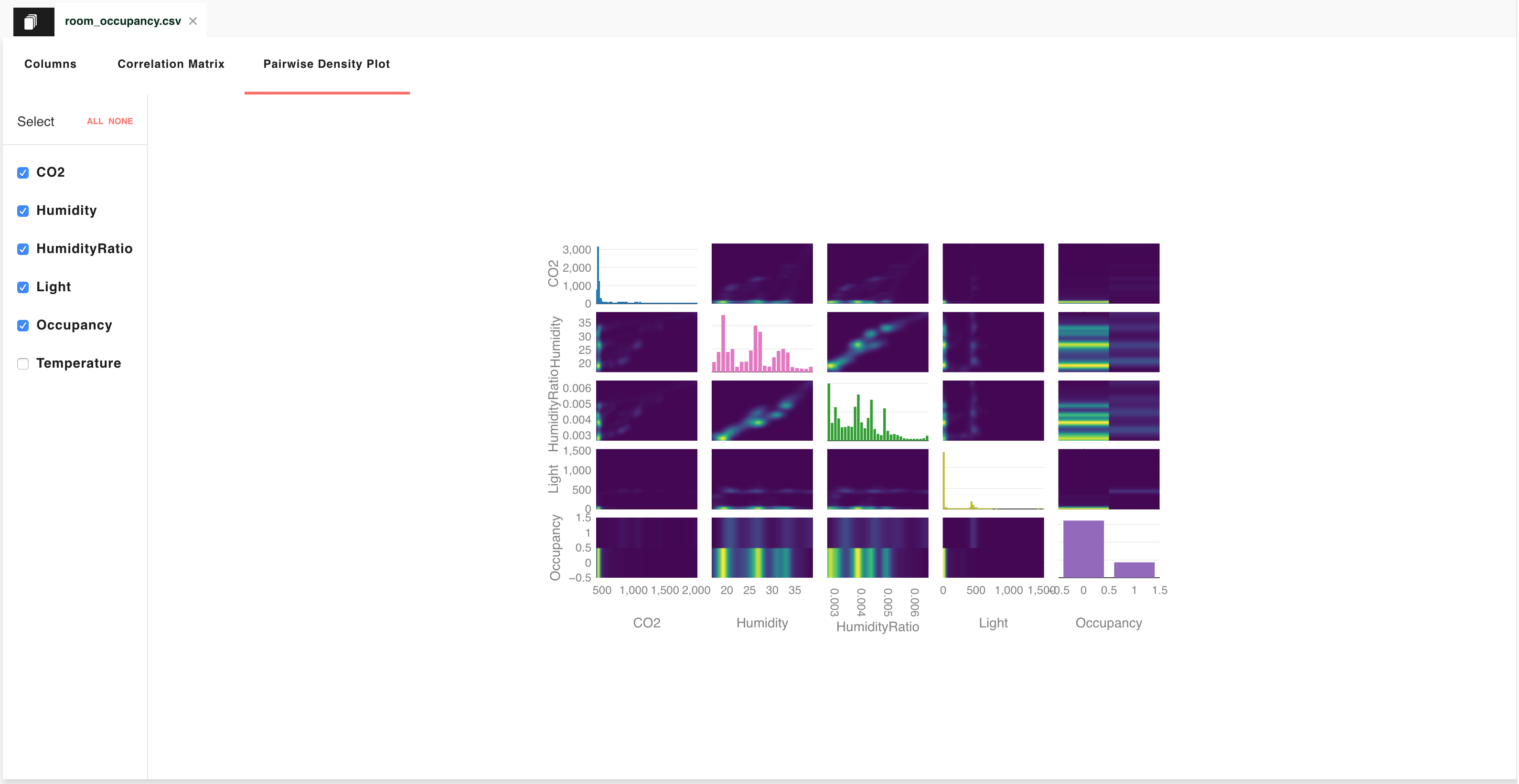
To be accurate, visualisations reported in this page are not scatter plots, but rather 2D Kernel Density Estimates (KDEs). These are approximations of joint Probability Density Functions (PDFs) for pairs of quantities in the dataset.