Experiments¶

Contents

Getting started
- Start tracking
- Customising
What can I log?
Multiple experiments
Using experiment tracking from Faculty Jobs
Getting data back out of experiments
Further reading

Increasingly, data science projects do not simply end with a few key takeaway conclusions, but result in trained machine learning models going into production. With these models taking ever more critical roles in organisations’ services and tooling, it’s important for us to track how models were created, know why a particular model was selected over other candidates, and be able to reproduce them when necessary.

Experiments in Faculty Platform makes it easy to keep track of this information. We’ve integrated MLflow, a popular open source project providing tooling for the data science workflow, into Faculty, requiring adding only minor annotations to your existing code.

For more information on why we introduced the experiment tracking feature, see our blog post on it.

Getting started ¶

Start tracking ¶

All you need to do to use MLflow and the experiment tracking feature in Faculty is to import the Python library and start logging experiment runs:

import mlflow

with mlflow.start_run():
    mlflow.log_param("gamma", 0.0003)
    mlflow.log_metric("accuracy", 0.98)

This will create a new run in the ‘Default’ experiment of the open project, which you can view in the Experiments screen:

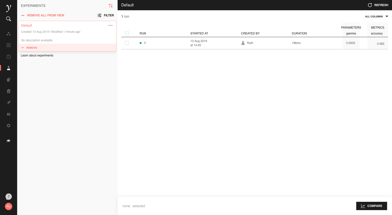
Clicking on the run will open a more detailed view:

Customising ¶

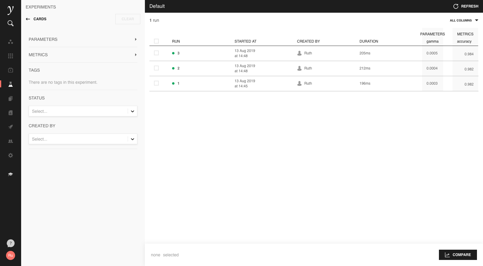
In the run history screen, we can customise the displayed columns in the top right, and sort columns by clicking on a column label.

With multiple runs, the ‘Filter’ option allows to filter runs based on logged information:

What can I log?¶

Model parameters, tags, performance metrics ¶

MLflow and experiment tracking log a lot of useful information about the experiment run automatically (start time, duration, who ran it, git commit, etc.), but to get full value out of the feature you need to log useful information like model parameters and performance metrics during the experiment run.

As shown in the above example, model parameters, tags and metrics can be logged. These are shown both in the list of runs for an experiment and in the run detail screen. In the following, more complete example, we’re logging multiple useful metrics on the performance of a scikit-learn Support Vector Machine classifier:

from sklearn import datasets, svm, metrics
from sklearn.model_selection import train_test_split
import mlflow

# Load and split training data
digits = datasets.load_digits()
data_train, data_test, target_train, target_test = train_test_split(
    digits.data, digits.target, random_state=221
)

with mlflow.start_run():

    gamma = 0.01
    mlflow.log_param("gamma", gamma)
    mlflow.set_tag("model", "svm")

    # Train model
    classifier = svm.SVC(gamma=gamma)
    classifier.fit(data_train, target_train)

    # Evaluate model performance
    predictions = classifier.predict(data_test)
    accuracy = metrics.accuracy_score(target_test, predictions)
    precision = metrics.precision_score(target_test, predictions, average="weighted")
    recall = metrics.recall_score(target_test, predictions, average="weighted")

    mlflow.log_metric("accuracy", accuracy)
    mlflow.log_metric("precision", precision)
    mlflow.log_metric("recall", recall)

If we then run the above code with different values of the gamma parameter, we can see and compare various runs and their metrics in the run history screen:

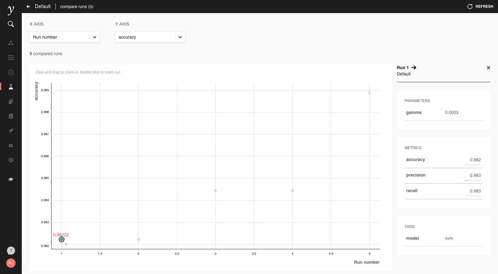
We can also compare runs visually by selecting runs and clicking ‘Compare’:

Models ¶

In addition to parameters and metrics, we can also log artifacts with experiment runs. These can be anything that can be stored in a file, including images and models themselves.

Logging models is fairly straightforward: first import the module in MLflow that corresponds to the model type you’re using, and call its log_model function. In the above example:

from sklearn import datasets, svm, metrics
from sklearn.model_selection import train_test_split
import mlflow
import mlflow.sklearn

# Load and split training data
# ...

with mlflow.start_run():

    gamma = 0.01
    mlflow.log_param("gamma", gamma)

    # Train model
    classifier = svm.SVC(gamma=gamma)
    classifier.fit(data_train, target_train)

    # Log model
    mlflow.sklearn.log_model(classifier, "svm")

    # Evaluate model performance
    # ...

Note

The following model types are supported in MLflow:

Keras (see mlflow.keras.log_model)
TensorFlow (see mlflow.tensorflow.log_model)
Spark (see mlflow.spark.log_model)
scikit-learn (see mlflow.sklearn.log_model)
MLeap (see mlflow.mleap.log_model)
H2O (see mlflow.h2o.log_model)
PyTorch (see mlflow.pytorch.log_model)

It’s also possible to wrap arbitrary Python fuctions in an MLflow model with mlflow.pyfunc.

The model will then be stored as artifacts of the run in MLflow’s MLmodel serialisation format. Such models can be inspected and exported from the artifacts view on the run detail page:

Context menus in the artifacts view provide the ability to download models and artifacts from the UI or load them into Python for further use.

The artifacts view also provides a “Register Model” feature, which enables structured and version controlled sharing of models. See Models for further documentation on this feature.

Artifacts ¶

It’s also possible to log any other kind of file as an artifact of a run. For example, to store a matplotlib plot in a run, first write it out as a file, then log that file as an artifact:

import os
import tempfile
import numpy
from matplotlib import pyplot
import mlflow

with mlflow.start_run():

    # Plot the sinc function
    x = numpy.linspace(-10, 10, 201)
    pyplot.plot(x, numpy.sinc(x))

    # Log as MLflow artifact
    with tempfile.TemporaryDirectory() as temp_dir:
        image_path = os.path.join(temp_dir, "sinc.svg")
        pyplot.savefig(image_path)
        mlflow.log_artifact(image_path)

The plot is then stored with the run’s artifacts and can be previewed and exported from the UI:

By the same mechanism, many types of files can be stored and previewed as part of an experiment run’s artifacts. A whole directory of artifacts can also be logged with mlflow.log_artifacts().

Multiple experiments ¶

Each Faculty project has a ‘Default’ experiment that runs will be stored in, unless configured otherwise. However, if you have a lot of experiment runs, you may wish to break them up into multiple experiments. To do this, just set the name of the experiment you wish to use in your notebook before starting any runs:

import mlflow

mlflow.set_experiment("SVM classifier")

with mlflow.start_run():
    # ...

If the experiment does not already exist, it will be created for you and appear as a new card in the run history screen:

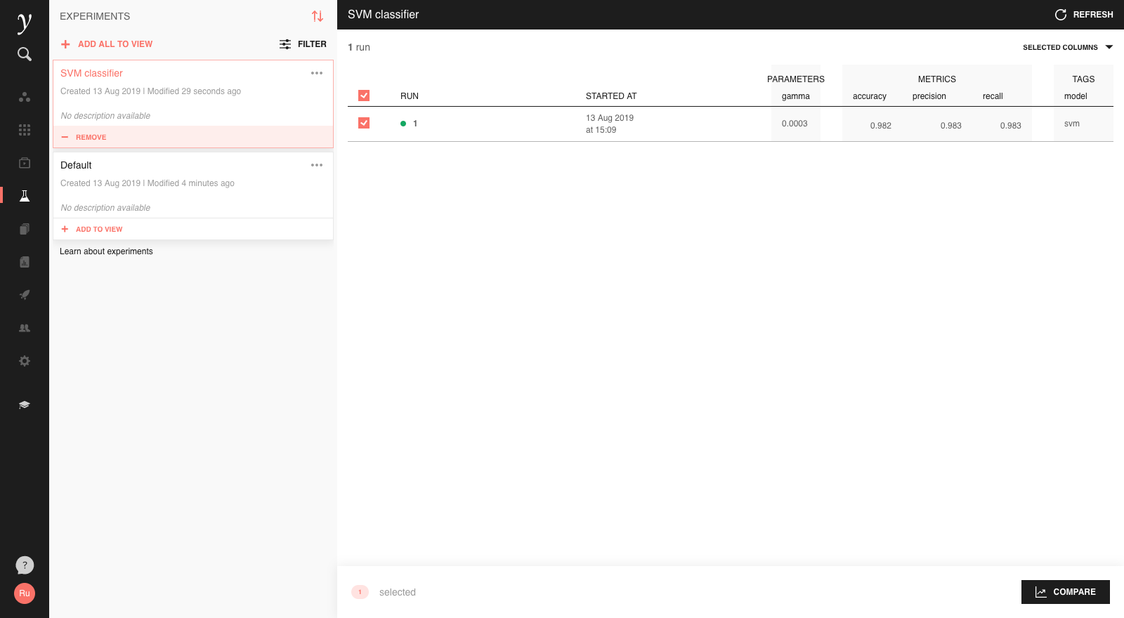
Tags can help to categorise runs within an experiment.

Using experiment tracking from Faculty Jobs ¶

It’s also possible to use experiment tracking with jobs. Just include the same MLflow tracking code as above in your Python script which gets run by the job, and experiments will be logged by the job automatically when run.

Experiments run from jobs will display the job and job run number used to generate them. Clicking on the job / run displayed in the experiment run will take you to the corresponding job, where you can see its logs and other runtime information.

Getting data back out of experiments ¶

Querying past experiments with MLflow ¶

Getting information about past experiment runs is straightforward with mlflow.search_runs. Calling it without any arguments will retrieve the runs for all runs in the active experiment as a pandas DataFrame:

import mlflow
df = mlflow.search_runs()

To retrieve runs for a different experiment, set the active experiment with mlflow.set_experiment as described above before calling search runs.

It’s also possible to filter runs with a SQL-like query with the filter_string argument. For example, to return only runs with a logged accuracy above 0.8:

import mlflow
df = mlflow.search_runs(filter_string="metric.accuracy > 0.8")

As with SQL, multiple filters can be combined with AND, OR and parentheses. Below is a more complete example:

import mlflow

query = """
   attribute.status = 'FINISHED' AND
   (metric.accuracy > 0.8 OR metric.f1_score > 0.8)
"""
df = mlflow.search_runs(filter_string=query)

The operators =, !=, >, >=, <, <=, AND and OR are supported. Valid fields to filter by are attribute.run_id, attribute.status, and param.<key>, metric.<key> and tag.<key> where <key> is replaced by the name of the param/metric/tag you wish to search by. If the key contains spaces or other special characters, wrap it in double quotes " or backticks `, e.g. metric.`f1 score`.

More information on mlflow.search_runs is available in the MLflow docs, however note that the Faculty implementation has some enhanced capabilities, in particular the ability to filter parameters by numeric value (and not just by string equality) and support for OR and parentheses.

Getting the full metric history ¶

The history of a metric during training of a model can be tracked by logging it multiple times during an experiment run. The metric history can be inspected by opening the run in the platform UI, but to get all the numbers out for further analysis or visualisation you can use the MLflow API.

To get the metric history, you’ll need to construct an MlflowClient and use its get_metric_history method, which takes the run ID and metric name. The run ID is displayed on the run page in the platform UI, and is also included in the output of mlflow.search_runs as described above.

from mlflow.tracking.client import MlflowClient

client = MlflowClient()
run_id = "ded7a224-3a51-4dcc-a6a0-36d994972878"
history = mlflow.get_metric_history(run_id, "accuracy")

get_metric_history returns a list of MLflow Metric objects, but you can easily convert to a more digestable output:

from datetime import datetime
import pandas as pd

history_df = pd.DataFrame(
    {
        "step": metric.step,
        "timestamp": datetime.fromtimestamp(metric.timestamp / 1000),
        "value": metric.value
    } for metric in history
)

Loading models ¶

To make predictions using a logged model from an experiment, we can use MLFlow’s mlflow.pyfunc.load_model interface. To illustrate how to use this functionality in the context of an app, assume we have trained a logistic regression to use a person’s age to predict whether they earn more than £50k, and logged it with an experiment run. To use the model for making predictions via an app, just load the model:

import mlflow.pyfunc
import pandas as pd

from flask import Flask, jsonify

# Instantiate Flask app
app = Flask(__name__)

# Load logged model using model ID and run ID
MODEL_URI = "logistic_regression"
RUN_ID = "f5121088-8b72-4fd7-a5fd-50653c988f4d"
MODEL = mlflow.pyfunc.load_model("runs:/{}/{}".format(RUN_ID, MODEL_URI))

# Interpret target values
TARGET_LABELS = {0: "< 50k", 1: "> 50k"}

# Use @app.route decorator to register run_prediction as endpoint on /
@app.route("/predict/<int:age>")
def run_prediction(age):
    df = pd.DataFrame({"age": [age]})

    # Run prediction
    prediction = MODEL.predict(df)[0]

    # Interpret prediction value
    prediction_label = TARGET_LABELS[prediction]

    return jsonify({"prediction": prediction_label})

# Run app
if __name__ == "__main__":
    app.run(port=5000, debug=True)

Finally, to get a prediction, send a GET request with a specific value for age, for example 55, to the server:

import requests

age = 55

requests.get("http://127.0.0.1:5000/predict/{}".format(age)).json()

This will decode the JSON response from the API and return a Python dictionary {"prediction": "< 50k"}.