Tutorial
Working with Opendata
[1]:
import time
import matplotlib.pyplot as plt
import pandas as pd

from IPython.display import display, HTML
from numpy import ceil

%matplotlib inline
Opendata gives you access to useful public datasets. It further implements automatic caching, which temporarely stores the dataset, making it readily available when loaded again.
To import the library faculty_extras.opendata, run:
[2]:
from faculty_extras import opendata
You can then view the datasets that are available in faculty_extras.opendata by means of opendata.ls(). This command accepts the optional argument prefix, which can be used to focus on a specific dataset. For instance, we will next analyse the census of the United Kingdom, provided in faculty_extras.opendata. To list the files that pertain to the UK census, we write:
[3]:
opendata.ls(prefix="uk_2011_census/")
[3]:
['uk_2011_census/census_by_outputarea.csv',
 'uk_2011_census/census_variable_info.csv',
 'uk_2011_census/outputarea_localauthority_mapping.csv',
 'uk_2011_census/outputarea_lsoa_msoa_mapping.csv',
 'uk_2011_census/outputarea_parliamentaryconstituency_mapping.csv',
 'uk_2011_census/postcode_outputarea_mapping.csv',
 'uk_2011_census/ukpostcodes.csv']
The caching functionality of faculty_extras.opendata makes repeated loading of a dataset considerably faster. For example, the first time we “read in” the UK census, the process takes about 5 seconds.
[4]:
# Measure dataset load time without cache
start = time.time()
census = opendata.load("uk_2011_census/census_by_outputarea.csv")
finish = time.time()
print("Time elapsed: {} seconds".format(finish - start))
Time elapsed: 5.321612354573562 seconds
By contrast, the second time the same dataset is loaded, the process takes only 0.2 seconds. The improvement in speed is achieved by temporarely saving the data into memory, so that any subsequent retrieval becomes straightforward.
[5]:
# Measure dataset load time with cache
start = time.time()
census = opendata.load("uk_2011_census/census_by_outputarea.csv")
finish = time.time()
print("Time elapsed: {} seconds".format(finish - start))
Time elapsed: 0.21984278934579285 seconds
Insights from Opendata
Let’s carry out some analysis on the census, in particular on data that concerns employment in different sectors of the economy. More specifically, we will compare employment figures for England, Northern Ireland, Scotland and Wales so as to understand the importance of different sectors towards the regional economies of the UK.
[6]:
# Load information about the census dataset
info = opendata.load("uk_2011_census/census_variable_info.csv")
[7]:
# Select information about industry-sector columns
sector_info = info[info["VariableSubDomain"] == "Industry Sector"]
[8]:
# Select OA column and industry-sector columns
selected_cols = ["OA"] + sector_info["VariableCode"].tolist()
sector = census[selected_cols]

# Set useful column names for dataframe 'sector'
selected_names = ["OA"] + sector_info["VariableTitle"].tolist()
sector.columns = selected_names
[9]:
# Consider England, Northern Ireland, Scotland and Wales individually
sector_england = sector[sector["OA"].str.startswith("E")]
sector_northern_ireland = sector[sector["OA"].str.startswith("N")]
sector_scotland = sector[sector["OA"].str.startswith("S")]
sector_wales = sector[sector["OA"].str.startswith("W")]
[10]:
# Calculate the number of individuals employed in each sector
tot_sector_england = sector_england.sum(numeric_only=True)
tot_sector_northern_ireland = sector_northern_ireland.sum(numeric_only=True)
tot_sector_scotland = sector_scotland.sum(numeric_only=True)
tot_sector_wales = sector_wales.sum(numeric_only=True)
[11]:
# Calculate the working population of each region
working_pop_england = tot_sector_england.sum()
working_pop_northern_ireland = tot_sector_northern_ireland.sum()
working_pop_scotland = tot_sector_scotland.sum()
working_pop_wales = tot_sector_wales.sum()
[12]:
# Calculate the number of people in each sector as
# a fraction of the working population in the region
ratio_sector_england = tot_sector_england / working_pop_england
ratio_sector_northern_ireland = (
    tot_sector_northern_ireland / working_pop_northern_ireland
)
ratio_sector_scotland = tot_sector_scotland / working_pop_scotland
ratio_sector_wales = tot_sector_wales / working_pop_wales
[13]:
def plot_sector(
    axis,
    sector,
    num_england,
    num_northern_ireland,
    num_scotland,
    num_wales,
    fontsize=14,
):
    """For a given sector, plot the number of individuals employed
    as a fraction of the working population in each UK region."""

    # Calculate % population employed in the sector for each region
    num_uk = [num_england, num_northern_ireland, num_scotland, num_wales]
    num_uk = [100.0 * n for n in num_uk]

    # Prepare title, xticks, and labels
    title = sector.replace("_", " ")
    xticks = [i for i in range(len(num_uk))]
    xticklabels = ["England", "N. Ireland", "Scotland", "Wales"]
    ylabel = "% population employed in this sector"

    # Plot
    axis.bar(xticks, num_uk)
    axis.set_title(title, size=fontsize)
    axis.set_xticks(xticks)
    axis.set_xticklabels(xticklabels, size=fontsize)
    axis.set_yticklabels(axis.get_yticks(), size=fontsize)
    axis.set_ylabel(ylabel, size=fontsize)
[14]:
%%javascript
// Disable autoscroll in subsequent Jupyter cells
IPython.OutputArea.prototype._should_scroll = function(lines) {
    return false;
}
We plot the number of individuals employed in various sectors of the UK economy. Data from different parts of the UK are compared, with each value expressed as a percentage of the working population in the region. This is to balance out the fact that England has a much larger population than Northern Ireland, Scotland and Wales.
[15]:
# List employment sectors
# to be visualised in plot
sectors = [
    "Information_and_communication",
    "Mining_and_quarrying",
    "Agriculture_forestry_and_fishing",
    "Human_health_and_social_work_activities",
    "Accommodation_and_food_service_activities",
    "Financial_and_insurance_activities",
]

# Specify overall width and
# height of the figure
num_subplots = len(sectors)
fig_width = 18
fig_height = 4 * num_subplots

# Specify the arrangement of subplots
num_subplot_cols = 2
num_subplot_rows = ceil(float(num_subplots) / num_subplot_cols)

# Initialise figure
fig = plt.figure(figsize=(fig_width, fig_height))

# Add subplots
for i, sector in enumerate(sectors):
    ax = fig.add_subplot(num_subplot_rows, num_subplot_cols, i + 1)
    plot_sector(
        ax,
        sector,
        ratio_sector_england[sector],
        ratio_sector_northern_ireland[sector],
        ratio_sector_scotland[sector],
        ratio_sector_wales[sector],
    )
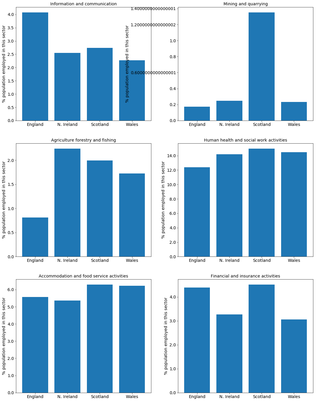
At this broad level, we see some interesting trends:
England is more heavily dependent on the service industries than the other countries, especially in the information and communication sectors.
“Mining and quarrying” is much larger in Scotland due to oil and gas extraction in the North Sea.
The agriculture, forestry and fishing industries have almost completely disappeared in England with almost sixteen times more people employed in health and social work activities.
Accommodation and food-service activities employ a greater fraction of the working population in Scotland and Wales. This is probably linked to the importance of tourism for the economy of these regions.
The census has many additional variables (age, gender, education), and a finer level of detail than “Country”. For example, Scotland shows a higher level of employment in financial and insurance services than England; however, if we were to further split England into regions, we would observe that these jobs show a significant concentration in London over the rest of the UK.